3.2.5. Inversion Input File

Both e3dmt.exe and e3dmt_iter.exe use the same input file. The lines of input file are as follows:

Line #	Description	Description
1	OcTree Mesh	path to octree mesh file
2	Observation File	path to observations file
3	1D Background Conductivity	1D background conductivity model
4	Initial Model	initial model
5	Reference Model	reference model
6	Background Susceptibility Model	background susceptibility model
7	Active Topography Cells	topography
8	Active Model Cells	active model cells
9	Cell Weights	additional cell weights
10	Face Weights	additional face weights
11	beta_max beta_min beta_factor	cooling schedule for beta parameter
12	alpha_s alpha_x alpha_y alpha_z	weighting constants for smallness and smoothness constraints
13	Chi Factor	stopping criteria for inversion
14	tol_nl mindm iter_per_beta	set the number of Gauss-Newton iteration for each beta value
15	tol_ipcg max_iter_ipcg	set the tolerance and number of iterations for Gauss-Newton solve
16	Reference Model Update	reference model
17	Hard Constraints	use SMOOTH_MOD or SMOOTH_MOD_DIFF
18	Bounds	upper and lower bounds for recovered model
19	BICG Parameters (Iterative .exe only)	set solver parameters for iterative inversion

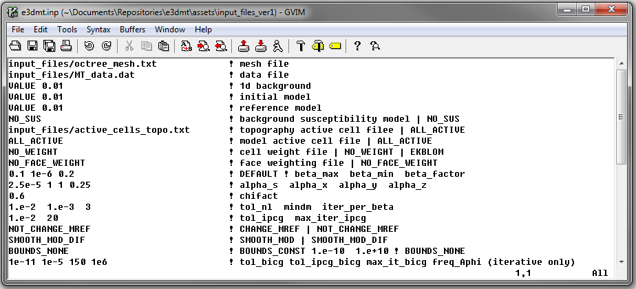
Fig. 3.6 Example input file for the inversion program (Download ).

3.2.5.1. Line Descriptions

• OcTree Mesh: file path to the OcTree mesh file

• Observation File: file path to the observed data file

• 1D Background Conductivity: The user may supply the file path to a 1D background conductivity model , or if a homogeneous background conductivity is being used, the user may enter “VALUE” followed by a space and a numerical value (example “VALUE 0.01”). The way the 1D model is used to determine the boundary conditions for solving the full 3D problem depends on the active topography cells options on line 7. Before continuing, the user is urged to read the section on boundary conditions.

Important

• The number of layers in the 1D model for E3DMT must equal the number of underlying mesh cells in the vertical direction. Thus if underlying mesh for the OcTree mesh is 1028 by 1028 by 512, the 1D model must have 512 layer conductivities.

• The boundary conditions computed using 1D models is only accurate when surface topography is minimal. In the case where surface topography is significant, it is suggested the user used E3DMT version 2.

• Initial Model: The user may supply the file path to an initial conductivity model. If a homogeneous conductivity value is being used for all active cells, the user can enter “VALUE” followed by a space and a numerical value; example “VALUE 0.01”.

• Reference Model: The user may supply the file path to a reference conductivity model. If a homogeneous conductivity value is being used for all active cells, the user can enter “VALUE” followed by a space and a numerical value; example “VALUE 0.01”.

• Reference Susceptibility Model: The user may supply the file path to a background susceptibility model. If the Earth is non-magnetic, the user may use the flag “NO_SUS”.

• Active Topography Cells: Here, the user can choose to specify the cells which lie below the surface topography. To do this, the user may supply the file path to an active cells model file or type “ALL_ACTIVE”. The active cells model has values 1 for cells lying below the surface topography and values 0 for cells lying above.

• Active Model Cells: Here, the user can choose to specify the model cells which are active during the inversion. To do this, the user may supply the file path to an active cells model file or type “ALL_ACTIVE”. The active cells model has values 1 for cells lying below the surface topography and values 0 for cells lying above. Values for inactive cells are provided by the background conductivity model.

• Cell Weights: Here, the user specifies whether cell weights are supplied. If so, the user provides the file path to a cell weights file If no additional cell weights are supplied, the user enters “NO_WEIGHT”.

• Face Weights: Here, the user specifies whether face weights are supplied. If so, the user provides the file path to a face weights file cell weights file. If no additional cell weights are supplied, the user enters “NO_FACE_WEIGHT”. The user may also enter “EKBLOM” for 1-norm approximation to recover sharper edges.

• beta_max beta_min beta_factor: Here, the user specifies protocols for the trade-off parameter (beta). beta_max is the initial value of beta, beta_min is the minimum allowable beta the program can use before quitting and beta_factor defines the factor by which beta is decreased at each iteration; example “1E4 10 0.2”. The user may also enter “DEFAULT” if they wish to have beta calculated automatically. See theory section for cooling schedule.

• alpha_s alpha_x alpha_y alpha_z: Alpha parameters . Here, the user specifies the relative weighting between the smallness and smoothness component penalties on the recovered models.

• Chi Factor: The chi factor defines the target misfit for the inversion. A chi factor of 1 means the target misfit is equal to the total number of data observations. For more, see the GIFtools cookbook .

• tol_nl mindm iter_per_beta: Here, the user specifies the number of Newton iterations. tol_nl is the Newton iteration tolerance (how close the gradient is to zero), mindm is the minimum model perturbation \(\delta m\) allowed and iter_per_beta is the number of iterations per beta value. See theory section for cooling schedule and Gauss-Newton update.

• tol_ipcg max_iter_ipcg: Here, the user specifies solver parameters. tol_ipcg defines how well the iterative solver does when solving for \(\delta m\) and max_iter_ipcg is the maximum iterations of incomplete-preconditioned-conjugate gradient. See theory on Gauss-Newton solve.

• Reference Model Update: Here, the user specifies whether the reference model is updated at each inversion step result. If so, enter “CHANGE_MREF”. If not, enter “NOT_CHANGE_MREF”.

• Hard Constraints: SMOOTH_MOD runs the inversion without implementing a reference model (essential \(m_{ref}=0\)). “SMOOTH_MOD_DIF” constrains the inversion in the smallness and smoothness terms using a reference model.

• Bounds: Bound constraints on the recovered model. Choose “BOUNDS_CONST” and enter the values of the minimum and maximum model conductivity; example “BOUNDS_CONST 1E-6 0.1”. Enter “BOUNDS_NONE” if the inversion is unbounded, or if there is no a-prior information about the subsurface model.

• BICG Parameters (omit line if using direct solver): In order, the user specifies values for tol_bicg, tol_ipcg_bicg, max_it_bicg and freq_Aphi; Example: 1E-10 1E-5 100 -1. These parameters are defined as follows:

  • tol_bicg: relative tolerance (stopping criteria) when solver is used during forward modeling; i.e. solves Eq. (2.11). Ideally, this number is very small (default = 1e-10).

  • tol_ipcg_bicg: relative tolerance (stopping criteria) when solver needed in computation of \(\delta m\) during Gauss Newton iteration; i.e. must solve Eq. (2.17) to solve Eq. (2.25). This value does not need to be as large as the previous parameter (default = 1e-5).

  • max_it_bicg: maximum number of BICG iterations (default = 100)

  • freq_Aphi: for frequencies below freq_Aphi, an SSOR preconditioner is constructed and used to solve the system more efficiently. However, the construction of preconditioners at each frequency may required a significant portion of additional RAM. To solve the system for all frequencies without using a preconditioner, set this value to a negative number (default = -1).

3.2.5.2. Details regarding boundary conditions

The way the 1D model is used to determine the boundary conditions for the full 3D problem depends on background conductivity (line 3) and the active topography cells (line 7). This can be explained as follows:

• Assume VALUE is used to define the 1D background model (line 3) and the flag ALL_ACTIVE is used to define active topography cells (line 7). Then the boundary conditions are obtained by solving the fields for a whole space. This approach is strongly discouraged!

• Assume VALUE is used to define the 1D background model (line 3) and an active cells model is used to define the active topography cells (line 7). Then the highest surface elevation in the active cells model is used as the surface elevation for the 1D model. Below this surface, the background conductivity is equal to the specified value. Above this surface, the background conductivity is set to air.

• Assume a 1D model defines the background conductivity (line 3) and the flag ALL_ACTIVE is used to define active topography cells (line 7). The top of the 1D model corresponds to the top of the OcTree mesh when solving the 1D problem. As a result, it is important to include air cells in the 1D model.

• Assume a 1D model defines the background conductivity (line 3) and an active cells model is used to define the active topography cells (line 7). Then the highest surface elevation in the active cells model is used as the surface elevation for the 1D model. The 1D problem is still solved and the top of the 1D model still corresponds to the top of the OcTree mesh. However, all layers above the surface are set to air regardless of the values specified in the 1D model.